Create benchmark plots#
Create the standard pyopmspe11 figures from the benchmark CSV files written in the previous lesson.
Command#
Use the same generation, reporting-grid, map-time, and write-interval settings used for the data workflow:
pyopmspe11 -i my_spe11b.toml -o my_spe11b -m plot -g all -r 50,1,15 -t 5 -w 1
How it works#
pyopmspe11 -mSelects the workflow.
plotreads existing benchmark CSV files and creates the standard figures without regenerating the deck, rerunning OPM Flow, or rewriting the data.pyopmspe11 -gSelects the data categories represented in the generated figures. Use the same value used when the CSV files were created.
pyopmspe11 -r,pyopmspe11 -t, andpyopmspe11 -wKeep the plotting configuration consistent with the reporting grid, spatial map times, and data intervals from the previous lesson.
Result#

CO2 mass mapped from the simulation grid to a 50 by 15 reporting grid (available at my_spe11b/figures/spe11b_tco2_2Dmaps.png).#
With subfolders enabled, simulation output is written under:
my_spe11b/
└── deck
└── flow
└── data
└── figures/
    ├── spe11b_arat_2dmaps.png
    ├── spe11b_co2_max_norm_res_2dmaps.png
    ├── spe11b_co2_mb_error_2dmaps.png
    ├── spe11b_cvol_2dmaps.png
    ├── spe11b_gden_2dmaps.png
    ├── spe11b_h2o_max_norm_res_2dmaps.png
    ├── spe11b_h2o_mb_error_2dmaps.png
    ├── spe11b_performance_detailed.png
    ├── spe11b_performance.png
    ├── spe11b_pressure_2dmaps.png
    ├── spe11b_sgas_2dmaps.png
    ├── spe11b_sparse_data.png
    ├── spe11b_tco2_2dmaps.png
    ├── spe11b_temp_2dmaps.png
    ├── spe11b_wden_2dmaps.png
    ├── spe11b_xco2_2dmaps.png
    ├── spe11b_xh2o_2dmaps.png
Customize figures with plopm#
The built-in plotting workflow creates standard figures. Use plopm when you need additional control over quantities, CSV columns, layouts, labels, colormaps, line styles, axis formatting, animations, or comparisons with OPM Flow output.
Install plopm with:
pip install git+https://github.com/cssr-tools/plopm.git
Create a nice figure:
plopm -i my_spe11b/flow/MY_SPE11B -v co2m -cbn 3 -cbf .1e -t 'CO$_2$ mass at the end of the simulation' -mv satnum -mt 1e4 -cbl 'kg' -c RdBu_r -yu km -xu km -xf .1f -yf .1f -fs 10,8 -fz 16
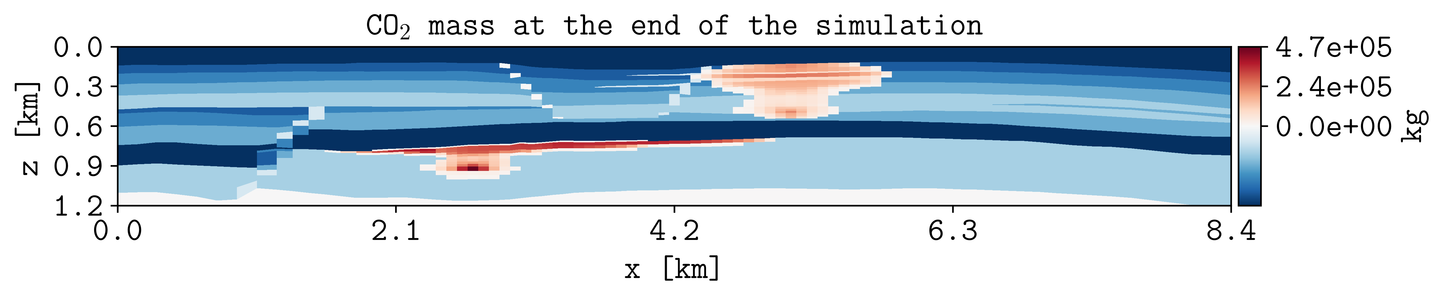
CO2 mass at the end of the simulation (figure created by plopm)#
See the plopm documentation for complete examples and command-line options.
Run the complete workflow#
Lessons 1 through 4 can be run in one command with -m all:
pyopmspe11 -i my_spe11b.toml -o my_spe11b -m all -g all -r 50,1,15 -t 5 -w 1
This generates the deck, runs OPM Flow, writes the benchmark CSV files, and creates the standard plots.
Next#
Continue with Modify the physical model. See Output folder for the output layout and Examples for additional visualization workflows.