Examples

Hello world

The examples folder contains configuration files with low grid resolution and shorter injection times (for initial testing of the framework). For example, by executing:

pyopmspe11 -i spe11b.toml -o spe11b -m all -g all -t 5 -r 50,1,15 -w 1

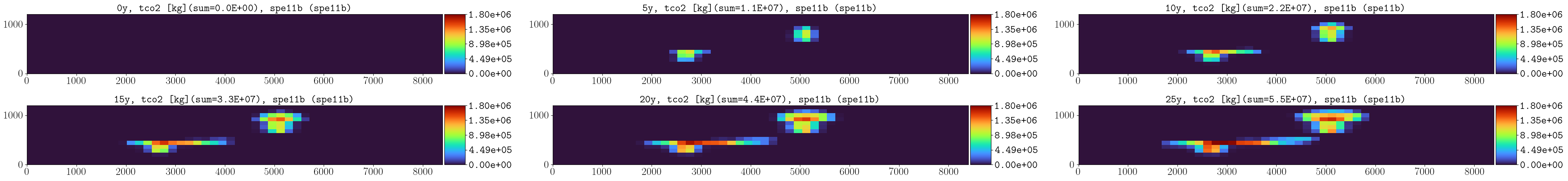
The following is the figure spe11b_tco2_2Dmaps, which shows the CO2 mass in the domain over time (i.e., the simulations results from the corner-point grid mapped to the equidistance reporting grid of 50 x 15 as defined by the -r flag). You can compare your example results to this figure to evaluate if your example ran correctly:

Note

To generate only the input files, this can be achieved by executing:

pyopmspe11 -i spe11b.toml -o spe11b -m deck

This does not required to have OPM Flow installed, and in principle should work in Windows without using the subsystem for Linux. Then, one could always generate a deck with the grid and all include files, and modify them in order to use other simulators different than OPM Flow.

Let us now change the model type from complete to immiscible, isothermal, and convective in line 7 of the configuration file, saving the toml file to these three model respectively. Then, we run the simulations:

pyopmspe11 -i immiscible.toml -o immiscible -m deck_flow_data -w 1
pyopmspe11 -i isothermal.toml -o isothermal -m deck_flow_data -w 1
pyopmspe11 -i convective.toml -o convective -m deck_flow_data -w 1

Here we have just set the framework to generate the deck, run the simulations, and generate the performance and sparse data (default value for -g). Then, to visualize the comparison between both runs, this can be achived by executing:

pyopmspe11 -c spe11b

The following are some of the figures generated in the compare folder:

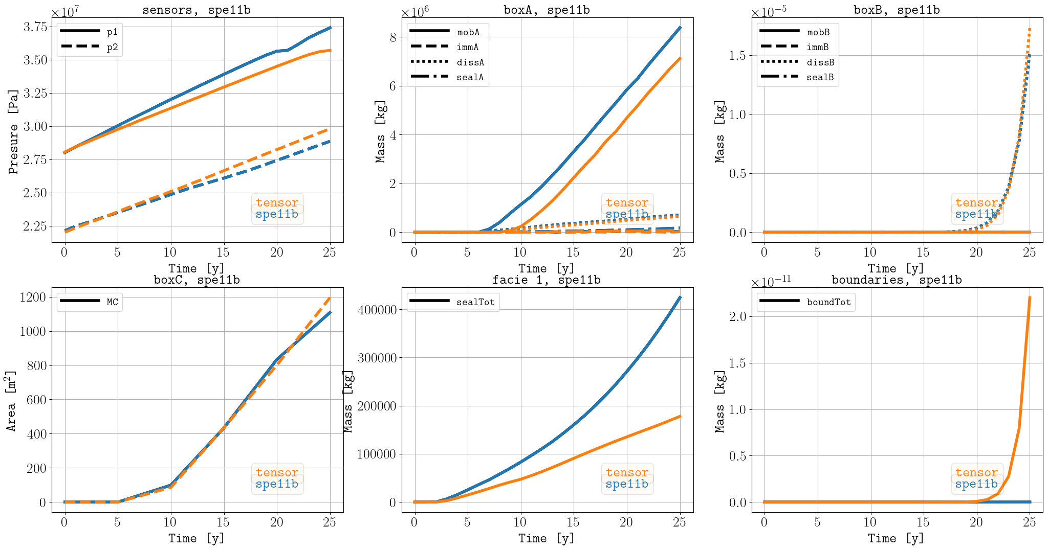
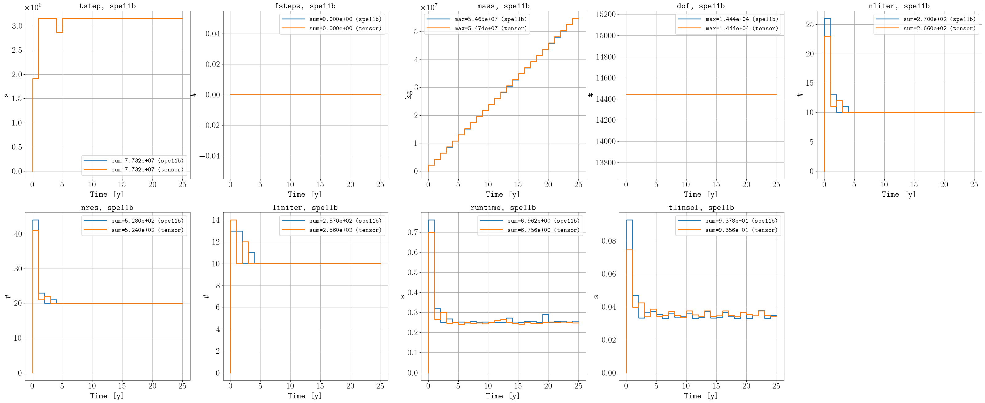
_images/spe11b_performance.png — The immiscible and isothermal simulations run faster since they have less dof.

Tip

This example shows how to use plopm to generate nice figures to compare simulation results (both from csv files (e.g., using the benchmark data set ) and from OPM Flow output files). You can install it by typing in the terminal:

pip install git+https://github.com/cssr-tools/plopm.git

This example uses a very coarser grid to run fast. See the benchmark section for finer grids.

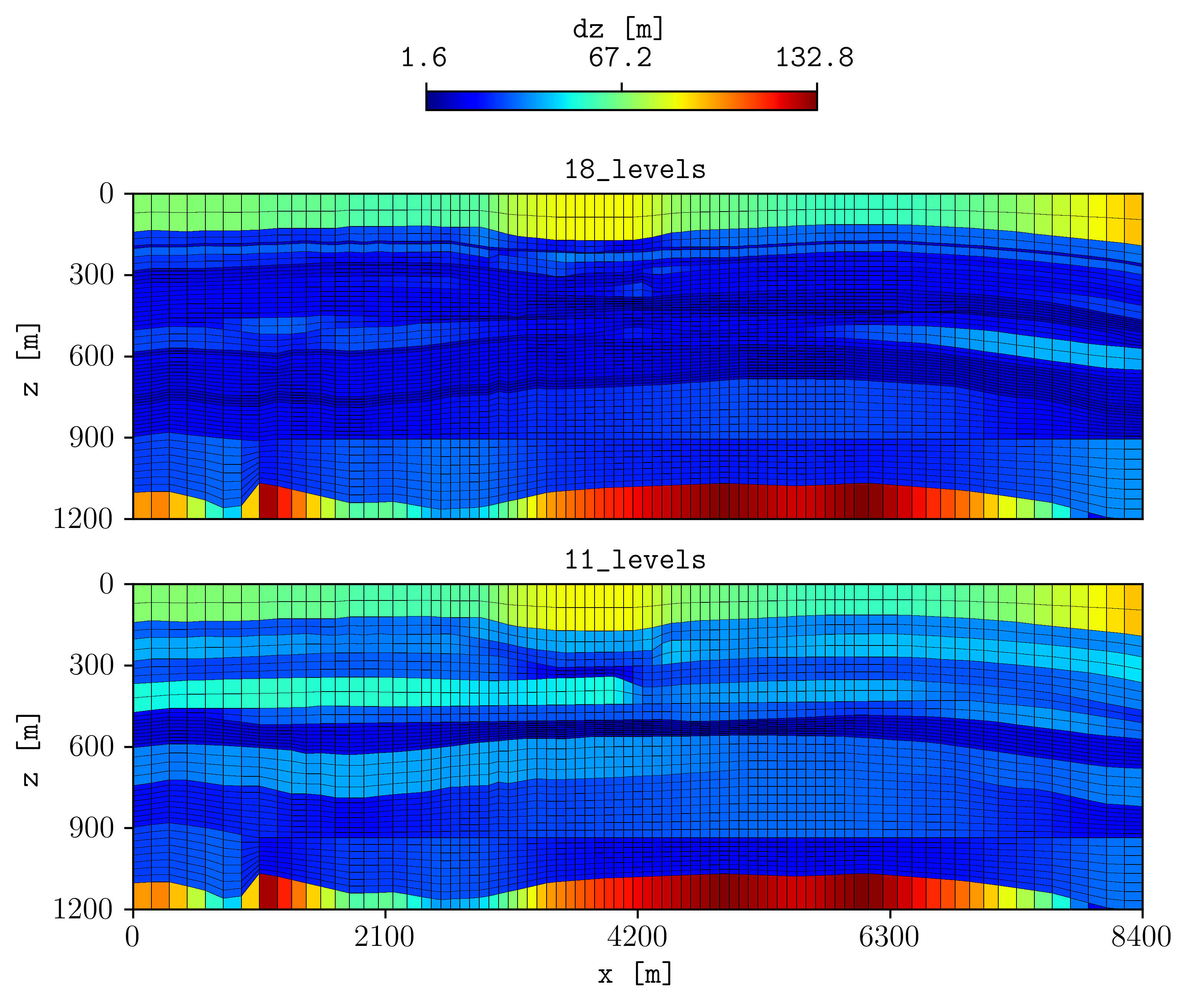
Cp grids (11 and 18 levels)

In a recent paper to history match the FluidFlower data using the laboratory images, a more regular coner-point grid was used consisting in 11 levels instead of 18 as the submitted results for the SPE11 benchmark. Then, the corner-point grid from that paper has been included in the pyopmspe11 tool. To use this corner-point grid, then one needs to give an array of size 11 for the variable “z_n” in the toml files. For example, in the spe11b.toml in the examples folder, setting z_n to [3, 2, 2, 2, 3, 2, 2, 8, 4, 8, 8, 1] and saving the configuration file as spe11b_11-levels.toml, running them (we add the flag -f 0 to generate the deck and simulation files in the output folder, i.e., no subfolders deck and flow), and using plopm to generate the figure:

pyopmspe11 -i spe11b.toml -o 18_levels -f 0
pyopmspe11 -i spe11b_11-levels.toml -o 11_levels -f 0
plopm -i '18_levels/18_LEVELS 11_levels/11_LEVELS' -v dz -subfigs 2,1 -delax 1 -z 0 -suptitle 0 -grid 'black,1e-2' -cbsfax 0.35,0.97,0.3,0.02

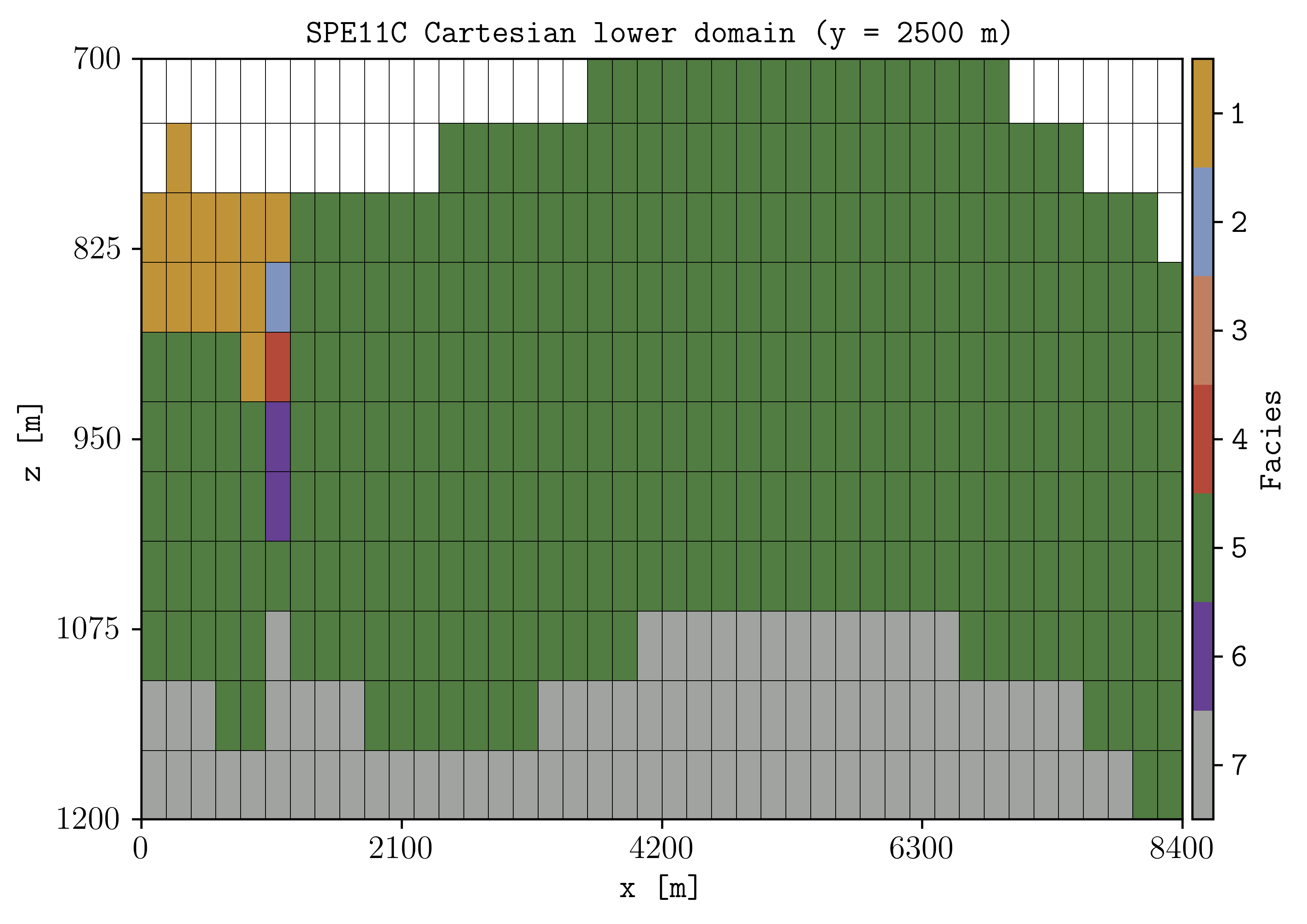
Localized lower domain

The flag -n lower results in the generation of files for the lower part (lower facie 5, removing the sealing facie 1) of the models. For example, using the spe11c.toml configuration file in the examples folder:

pyopmspe11 -i spe11c.toml -o lower_domain -f 0 -n lower
plopm -i lower_domain/LOWER_DOMAIN -s ,14, -y '[1200,700]' -z 0 -grid 'black,1e-2' -t "SPE11C Cartesian lower domain (y = 2500 m)" -clabel "Facies" -c '161;163;160 101;64;147 81;124;66 181;73;57 193;127;97 127;148;191 193;147;56' -cticks '[7, 6, 5, 4, 3, 2, 1]' -v 'pvtnum - 1 - satnum'

_images/lower_domain_pvtnum-1-satnum_i%2C14%2Ck_t5.png

See the convergence for using the localized domain in the SPE11B corner-point grid case.