Derived Results - Geomechanical
ResInsight computes several derived results. In this section we will explain what they are, and briefly how they are calculated.
Derived Geomechanical results
ResInsight calculates several of the presented geomechanical results based on the native results present in the odb-files.
Relative Results (Time Lapse Results)
ResInsight can calculate and display relative results, sometimes also referred to as Time Lapse results. When enabled, every result variable is calculated as:
$Value_{[t-b]} = Value_{[t]} - Value_{[b]}$
where:
- $b$ is the base time step,
- $t$ is the current time step
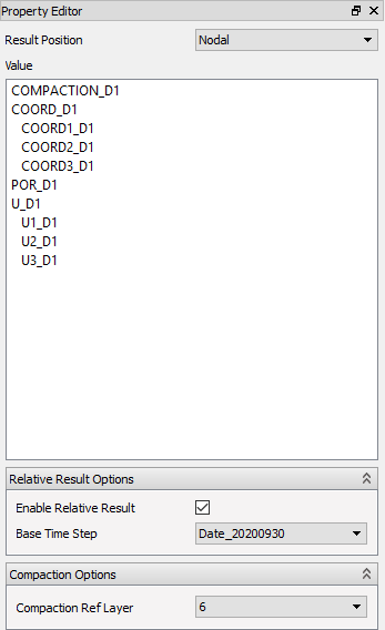
Select the appropriate Base Time Step option in the Difference Options group to enable the time lapse result.
Note: Relative Results calculated based on Gamma values and Stress Anisotropy are calculated slightly differently:
Gamma:
$Gamma_{i[t-b]} = \frac{ST_{i[t]} - ST_{i[b]}}{ POR_{[t]} - POR_{[b]} }$
Stress Anisotropy:
$SA_{ij[t-b]} = 2 * \frac{(ST_{i[t]} - ST_{i[b]}) - (ST_{j[t]} - ST_{j[b]})}{(ST_{i[t]} - ST_{i[b]}) + (ST_{j[t]} - ST_{j[b]})}$
Derived Result Fields
The calculated result fields are:
- Nodal
- COMPACTION (Magnitude of compression)
- Element Nodal and Integration Points
- ST (Total Stress)
- All tensor components
- Principals, with directions ($S_iinc, S_iazi$)
- STM (Mean total stress)
- Q (Deviatoric stress)
- Gamma (Stress path)
- SE (Effective Stress)
- All tensor components
- Principals, with directions
- SEM (Mean effective stress)
- SFI
- FOS
- DSM
- E (Strain)
- All tensor components
- EV (Volumetric strain)
- ED (Deviatoric strain)
- ST (Total Stress)
- Element Nodal On Face
- Plane
- Pinc (Face inclination angle)
- Pazi (Face azimuth angle)
- Transformed Total and Effective Stress
- SN (Stress component normal to face)
- TP (Total in-plane shear)
- TPinc (Direction of TP)
- TPH ( Horizontal in-plane shear component )
- TPQV ( Quasi vertical in-plane shear component )
- FAULTMOB
- PCRIT
- Plane
Definitions of Derived Results
In this text the label Sa and Ea will be used to denote the unchanged stress and strain tensor respectively from the odb file.
Components with one subscript denotes the principal values 1, 2, and 3 which refers to the maximum, middle, and minimum principals respectively.
Components with two subscripts however, refers to the global directions 1, 2, and 3 which corresponds to X, Y, and Z and thus also easting, northing, and depth.
- Inclination is measured from the downwards direction
- Azimuth is measured from the Northing (Y) Axis in Clockwise direction looking down.
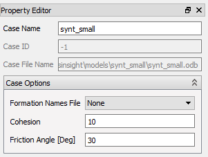
Case Constants
Two constants can be assigned to a Geomechanical case:
- Cohesion
- Friction angle
In the following they are denoted s0 and fa respectively. Some of the derived results use these constants, that can be changed in the property panel of the Case.
COMPACTION
Compaction is the difference in vertical displacement (U3) between a grid node and a specified reference K layer. The reference K layer is specified in the property editor.
For each node n in the grid, a node nref in the reference K layer is found by vertical intersection from the node n.
$ If (Depth_n <= Depth_{nref}) $
$ \space \space COMPACTION_n = -(U3_n - U3_{nref})$
$ else $
$\space \space COMPACTION_n = -(U3_{nref} - U3_n )$
ST - Total Stress
$ST_{ii} = -Sa_{ii} + POR (i= 1,2,3)$
We use a value of $POR=0.0$ where it is not defined.
$ST_{ij} = -Sa_{ij} (i,j = 1,2,3 \text{ and i $\ne$ j})$
$Sa_{ii}$ and $Sa_{ij}$ are the stresses calculated by Abaqus.
$ST_i = \text{Principal value i of ST}$
STM - Total Mean Stress
$STM = \frac{ST_{11} + ST_{22} + ST_{33}}{3} $
Q - Deviatoric Stress
$Q = \sqrt {\frac{3}{2} * ((ST_1 - STM)^2 + (ST_2 - STM)^2 + (ST_3 - STM)^2 }$
DPN - Shear Slip Indicator
Excess pore pressure parameter is defined as
$DPN = \frac{P_p - P_0} { \sigma_v - P_0 }$
Where:
- $P_0$ is hydrostatic pore pressure,
- $P_p$ is pore pressure (at the time of the incident) and
- $\sigma_v$ total vertical stress ($ ST_{33} $).
Hydrostatic pore pressure is
$ P_0 = \rho_w * TVDMSL * g $
Where:
- $\rho_w$ is (average) density of formation water (default = 1.03),
- TVDMSL is true vertical depth mean sea level and
- $g$ is gravity.
Gamma - Stress Path
$Gamma_{ii} = \frac{ST_{ii}} {POR} (i= 1,2,3) $
$Gamma_{i} = \frac{ST_{i}} {POR} $
In these calculations we set Gamma to undefined if abs(POR) > 0.01 MPa.
SE - Effective Stress
$SE_{ij} = -Sa_{ij} (i,j = 1,2,3 \text{ where POR is defined})$
where $Sa_{ij}$ is the stress calculated by Abaqus.
$SE_i = \text{Principal value i of SE} $
SEM - Effective Mean Stress
$SEM = \frac{SE_{11} + SE_{22} + SE_{33}} {3} $
SA - Stress Anisotropy
$SA_{ij} = 2 \frac{ST_{i} - ST_{j}}{ ST_{i} + ST_{j}} (i,j = 1,2,3 \text{ and i $\lt$ j})$
The same expressions are available for effective stresses (where SE replaces ST in the equation above).
SFI
$$SFI = \frac{\frac{S0}{tan(fa)} + 0.5 * (SE_1 + SE_3) * sin(fa)} {0.5*(SE_1-SE_3)} $$
DSM
$DSM = \frac{tan(\rho)} {tan(fa)} $
where
$$ \rho = 2 * (arctan (\sqrt \frac{ SE_1 + a} {SE_3 + a}) \space – \frac {\pi} {4}) $$ $$ a = \frac {s0} {tan(fa)} $$
FOS
$FOS = \frac{1}{DSM}$
E - Strain
$E_{ij} = -Ea_{ij}$
EV - Volumetric Strain
$EV = E_{11} + E_{22} + E_{33} $
ED - Deviatoric Strain
$ED = 2*\frac {E1-E3} {3} $
Element Nodal On Face
For each face displayed, (might be an element face or an intersection/intersection box face), a coordinate system is established such that:
- Ez is normal to the face, named N - Normal
- Ex is horizontal and in the plane of the face, named H - Horizontal
- Ey is in the plane pointing upwards, named QV - Quasi Vertical
The stress tensors in that particular face are then transformed to that coordinate system. The following quantities are derived from the transformed tensor named TS in the following:
SN - Stress component Normal to face
$SN = TS_{33}$
TPH - Horizontal in-plane shear component
$TPH = TS_{31} = TS_{ZX} $
TNQV - Horizontal in-plane shear component
$TPQV = TS_{32} = TS_{ZY}$
TP - Total in-plane shear
$TP = \sqrt {(TPH^2 + TPQV^2)} $
TPinc - Direction of TP
Angle of the total in-plane shear relative to the Quasi Vertical direction
$TPinc = acos (\frac {TPQV} {TP}) $
FAULTMOB
$FAULTMOB = \frac{TP}{tan(frictionAngle) * (TS_{ZZ} + \frac{cohesion}{tan(frictionAngle)} )}$
PCRIT
$PCRIT = TS_{ZZ} - \frac{TP}{tan(frictionAngle)} $
Pinc and Pazi - Face Inclination and Azimuth
These are the directional angles of the face-normal itself.
Pore Compressibility
Pore Compressibility
Pore compressibility between a reference state and the current stress state is defined as:
$ C_{p} = -\frac{ \alpha \Delta\epsilon_{vol}}{ \Delta P_p \phi_0} + \frac{1}{K_s} ( \frac{ \alpha } { \phi_0 } - 1) $
Where:
- $ \alpha $ is the Biot coefficient,
- $ \Delta\epsilon_{vol} $ is volumetric strain change (EV in ResInsight) between current state and reference state,
- $ \phi_0 $ is porosity on the Geostatic step,
- $ \Delta P_p $ is change in pore pressure between current state and reference state,
- $ K_s $ bulk modulus for the solid material (grain).
The Biot porelastic coefficient ($\alpha$) defines the compressibility of sand grains: $\alpha = 1.0$ for incompressible grains, and $\alpha < 1.0$ for compressible grains. $\alpha$ is not used for the initial (Geostatic) time step. The default value is 1.0, but values per element can be imported as an element property table.
The bulk modulus for solid material is defined as:
$ K_s = \frac{ K_{fr} }{ 1 - \alpha}, K_{fr} = \frac{ E }{ 3(1-2\nu)} $
Where:
- $ E $ is the elastic modulus (Young’s modulus) from element property table MODULUS.
- $ \nu $ is Poisson’s ratio imported from element property table RATIO.
Vertical Compressibility
$ C_{v} = - \frac{ \Delta\epsilon_{\nu}}{ \alpha \Delta P_p } $
$ \Delta\epsilon_\nu $ is the vertical strain change between current state and reference state (E33 in ResInsight).
Vertical Compressibility Ratio
$ C_{vr} = \frac{ C_v E(1-\nu) } { (1+\nu) ( 1 - 2\nu) } $
Vertical Compression Ratio is the ratio between the real vertical compression and the compression in a uniaxial strain case. All parameters are described above.
Porosity and Permeability
Porosity
Porosity change is defined as either total change in porosity between initial (geostatic) state and current state, or change in porosity between a reference state and the current state $ \Delta\phi $. The latter is given as
$ \Delta\phi = \phi_0(C_p \Delta P_p + \Delta\epsilon_{vol}) $
Here, $\Delta\phi_0$ is found from this equation with the reference state being the initial state (geostatic). The current porosity is then given as
$ \phi = \phi_0 + \Delta\phi_0 $
with $ \phi_0 $ being the porosity at the initial state, $\Delta\phi_0$ is porosity change between initial (geostatic) state current, $C_p$ is pore compressibility (between reference and current state), $\Delta P_p$ is change in pore pressure and $\Delta\epsilon_{vol}$ is volumetric strain change.
Initial Porosity
Porosity at the initial state:
$ \phi_0 = \frac{VOIDR} {1 + VOIDR} $
Where:
- VOIDR is void ratio from Abaqus.
Permeability
An expression for permeability is taken from Petunin (2011).
$ k = k_0( \frac{\phi}{\phi_0} )^A $
Where:
- $k_0$ is the permeability at the initial state (unit: mD),
- $\phi$ is porosity at current state,
- $\phi_0$ is initial porosity,
- $A$ is a constant
Mud Weight Window
Mud Weight Window (MWW) represents the difference between the minimum and the maximum possible mud weight between specific formation layers representing top and base of a fictitious well section.
To find MWW a two step procedure is needed:
- first find the limits per element,
- determine the MWW for each element based on the vertical column.
Finding Upper and Lower Mud Weight Limit
The upper mud weight limit (UMWL) and lower mud weight limit (LMWL) is found for each element intersected by the fictitious well. The UMWL is either the fracture gradient (FG) or minimum horizontal stress (SHmin) for both sand and shale. The LMWL is defined as the maximum of shear fracture gradient (SFG) and/or pore pressure in shale, and as pore pressure in sand.
The calculations for fracture gradient and shear fracture gradient, and the needed input, are described in detail in Well Bore Stability Plots.
Mud Weight Window
Thereafter, the combined use of mud weight limits for all elements between the top and base (for a given IJ) determines the MWW parameters as will be further described below.
A reference element index ($K_{ref}$) represents the base or the top of the fictitious well. Then for a set of elements with i = I, j = J and k = K to $K_{ref}$ the maximum LWML and the minimum UWML must be found from these element values. Then the difference between the two defines the MWW parameter.
Thus for a vertical stack of elements $element_{ijk} = K \to K_{ref}$, $MWW_{ijk}$ is given as
$ MWW_{ijk} = maximum(LMWL) - minimum(UMWL) (k = K \to K_{ref}) $
Similar calculations are made below the reference layer, but then with the reference layer as the top layer.
In addition to the MWW parameter, the mud weight representing the middle of the drilling window (MWM) is calculated if MWW > 0. Otherwise, MWM should is undefined.