Result Inspection
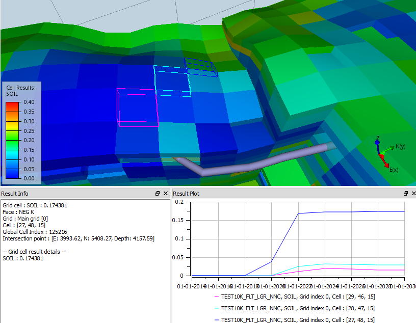
The results mapped on the 3D model can be inspected in detail by left clicking cells in the 3D view. The selected cells will be highlighted, text information displayed in the Result Info docking window, and the time-history values plotted in the Result Plot, if available.
The values along the different K-layers is available in the Depth Plot
Note
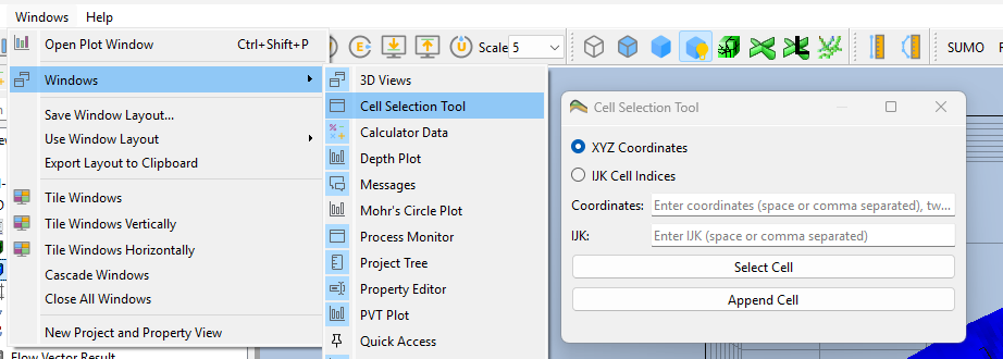
Visibility of the docking widows can be controlled from the Windows menu.
Result Info
Clicking cells will display slightly different information text based on the case type as described in the following tables.
Selection of cells can now be done by entering IJK or a UTM coordinate. This feature is available from the Windows menu, Cell Selection Tool.
Eclipse Model
| Geometry | Description |
|---|---|
| Reservoir cell | Displays grid cell result value, cell face, grid index and IJK coordinates for the cell. The intersection point coordinates is also displayed. Additional result details are listed in the section – Grid cell result details – |
| Fault face | Displays the same info as for a Reservoir cell. In addition the section – Fault result details – containing Fault Name and Fault Face information. |
| Fault face with NNC | Displays the same info as Fault face, except the Non Neighbor Connections (NNC) result value is displayed instead of grid cell value. Information added in section – NNC details – is geometry information of the two cells connected by the NNC. |
| Formation names | Displays name of formation the cell is part of |
Geomechanical Model
| Name | Description |
|---|---|
| Closest result | Closest node ID and result value |
| Element | Element ID and IJK coordinate for the element |
| Intersection point | Location of left-click intersection of the geometry |
| Element result details | Lists all integration point IDs and results with associated node IDs and node coordinates |
| Formation names | Displays name of formation the cell is part of |
Result Plot
The result values of the selected cells for all time steps are displayed in the docking window Result Plot as one curve for each cell.
Additional curves can be added to the plot if CTRL-key is pressed during picking. The different cells are highlighted in different colors, and the corresponding curve is colored using the same color.
To clear the cell-selection, left-click outside the visible geometry.
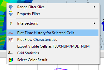
These curves can also be displayed in a summary plot in the main plot window using the right-click menu option “Plot Time History for Selected Cells”.
Adding the Curves to a Summary Plot
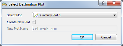
The time history curves of the selected cells can be added to a Summary Plot by right-clicking in the Result Plot or in the 3D View.
A dialog will appear to prompt you to select an existion plot, or to create a new one.
PVT Plot
Show the PVT Plot window by selecting Windows -> PVT Plot. When it is turned on, it will only be visible when the active view is a view of a reservoir simulation case.
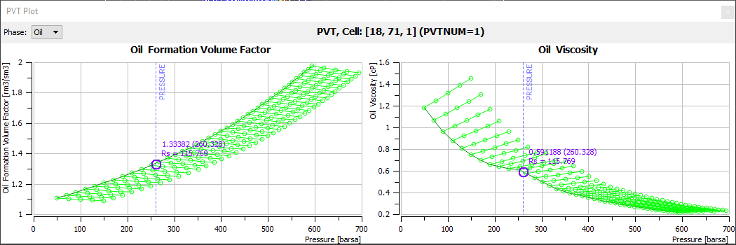
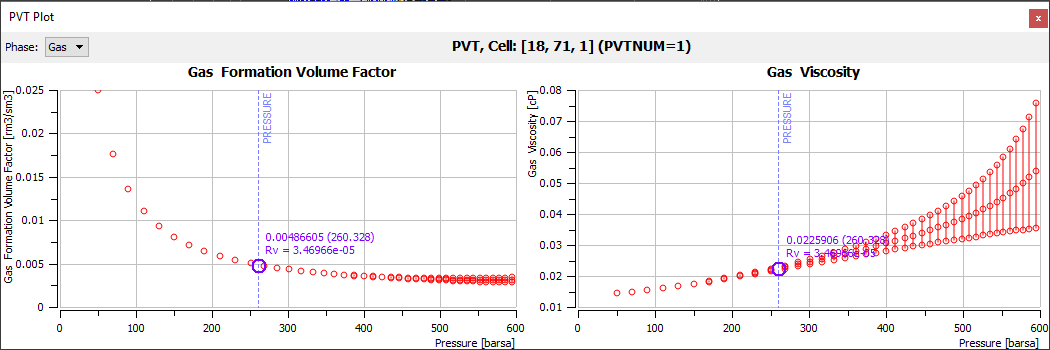
The PVT plot window shows two plots, based on PVTNUM in the selected cell. One plots Phase Formation Volume Factor and the other plots Phase Viscosity, both against pressure. The Phase can be either oil or gas, and can be selected in the top left corner of the window.
Pressure for the selected cell, at the current time step, is marked on the plot as a vertical line, and a large circle marks the scalar value of the cell (formation volume factor/viscosity). RV for the selected cell is also shown.
Relative Permeability Plot
Show the Relative Permeability Plot window by selecting Windows -> Relative Permeability Plot. When it is turned on, it will only be visible when the active view is a view of a reservoir simulation case.
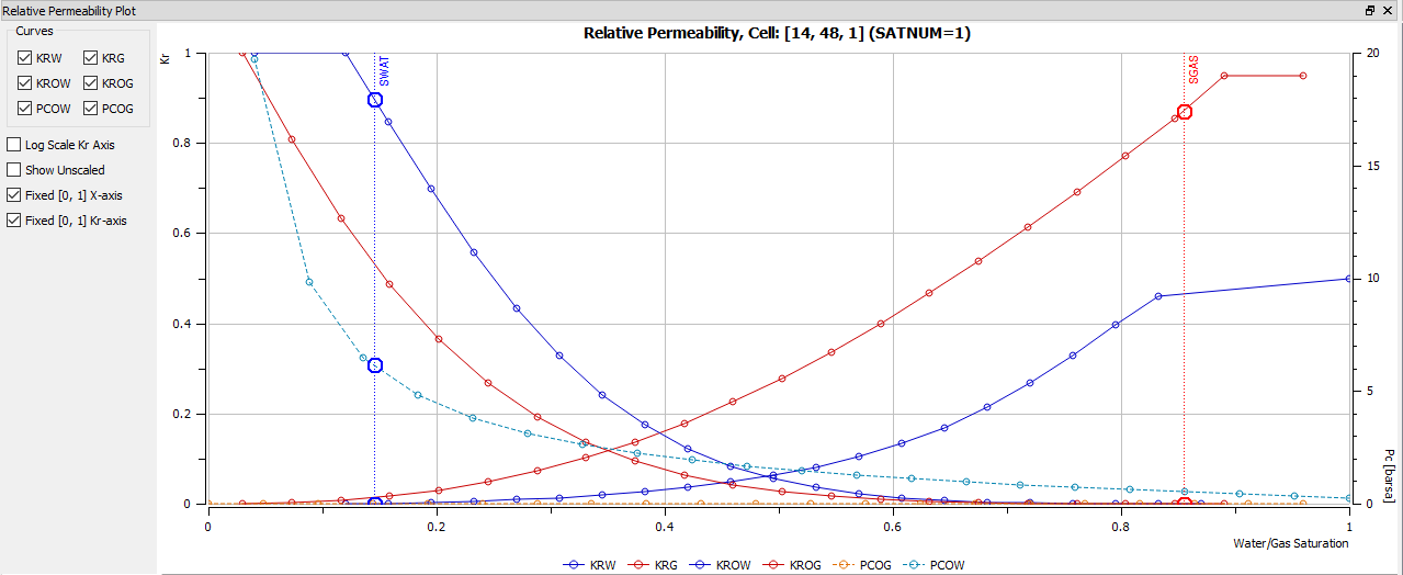
The Relative Permeability Plot window shows up to six curves, based on SATNUM in the selected cell. The curves can be turned on/off in the top left corner of the window, and they are described in the following table:
| Name | Description | Axis |
|---|---|---|
| KRW | Relative permeability water | KR (Left) |
| KRG | Relative permeability gas | KR (Left) |
| KROW | Relative permeability oil water | KR (Left) |
| KROG | Relative permeability oil gas | KR (Left) |
| PCOW | Capilar pressure oil water | PC (Right) |
| PCOG | Capilar pressure oil gas | PC (Right) |
Saturation of water and gas in the selected cell, at the current time step, are annotated in the plot by a blue and orange vertical line, respectively. The intersections between the lines and the relevant curves are marked with large circles.
| Option | Description |
|---|---|
| Log Scale Kr Axis | Enable logarithmic Kr-axis |
| Show Unscaled | Display curves unscaled |
| Fixed [0, 1] X-axis | Use a fixed range on X-axis |
| Fixed [0, 1] Kr-axis | Use a fixed range on Kr-axis |
Mohr’s Circle Plot (Geo Mechanical Models Only)
Show the Mohr’s Circle Plot window by selecting Windows -> Mohr’s Circle Plot. When it is turned on, it will only be visible when the active view is a view of an Geo Mech case.
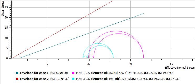
The Mohr’s circle plot shows three circles representing the 3D state of stress for a selected cell. In addition, it shows the envelope, calculated from the cohesion and friction angle given in the geo mechanical view’s property editor. Several sets of circles and envelopes can be added by selecting more than one cell in any view (as in image above).